CIFAR-10에서 ResNet-18(직접구현) vs VGG19-BN: 최적화 안정성, 수렴 특성, 일반화 성능 비교
0. 목표와 설계 개요
목표
Residual Learning의 실제 이점을 검증하기 위해, torchvision 미사용 직접 구현 ResNet-18을 CIFAR-10에 맞춰 학습하고, VGG19-BN과 동일한 학습 조건에서 성능·수렴 특성을 정량/정성 비교한다.
가설
1. ResNet은 F(x)+x의 identity 경로로 인해 깊이가 같아도 학습이 더 안정되고 수렴이 빠르다.
2. 동일 증강/스케줄에서 ResNet-18은 더 적은 파라미터로도 더 높은 테스트 정확도를 달성한다.
실험 설계
- 데이터 : CIFAR-10, 표준 정규화 + RandomCrop(32, pad=4), RandomHorizontalFlip
- 옵티마이저/스케줄: SGD(m=0.9, wd=5e-4), MultiStepLR([50,75], γ=0.1) → 0.1 → 0.01 → 0.001
- 비교 : 동일 전처리/배치(128)/에폭(100)/스케줄
| Model | Test Loss | Test Acc(%) | #Params(M) | Best Val(%) |
| ResNet-18 | 0.1937 | 94.99 | 11.17 | 94.99 |
| VGG19(BN) | 0.3345 | 92.87 | 38.96 | 92.87 |


1. 구현 (torchvision 미사용 ResNet-18)
1.1 CIFAR-10에 맞춘 ResNet-18 설계
- Stem: ImageNet 스타일(7×7 Conv + MaxPool)을 생략하고, CIFAR-10 해상도(32×32)에 맞춰
Conv3×3(3→64, stride=1, pad=1) → BN → ReLU로 간결화. - BasicBlock (Residual Unit)
- Conv3×3(s) → BN → ReLU → Conv3×3(1) → BN
- 입력/출력 채널 또는 stride가 달라질 때만 1×1 Conv + BN으로 downsample
- 출력: ReLU( F(x) + identity )
- Stage 구성: 채널 [64, 128, 256, 512], 블록 수 [2,2,2,2], stage 2~4의 첫 블록만 stride=2
- 헤드: AdaptiveAvgPool2d(1,1) → FC(512→10)
- 초기화: Kaiming Normal(He) for Conv, BN γ=1/β=0
# 데이터 전처리

transform_train = T.Compose([
    T.RandomCrop(32, padding=4),
    T.RandomHorizontalFlip(),
    T.ToTensor(),
    T.Normalize([0.4914,0.4822,0.4465],[0.2470,0.2435,0.2616]),
])
transform_test = T.Compose([
    T.ToTensor(),
    T.Normalize([0.4914,0.4822,0.4465],[0.2470,0.2435,0.2616]),
])

train_ds = torchvision.datasets.CIFAR10('./data', train=True,  download=True, transform=transform_train)
test_ds  = torchvision.datasets.CIFAR10('./data', train=False, download=True, transform=transform_test)
train_loader = DataLoader(train_ds, batch_size=128, shuffle=True,  num_workers=2, pin_memory=True)
test_loader  = DataLoader(test_ds, batch_size=128, shuffle=False, num_workers=2, pin_memory=True)
# BasicBlock

class BasicBlock(nn.Module):
    expansion = 1
    def __init__(self, in_channels, out_channels, stride=1, downsample=None):
        super().__init__()
        self.conv1 = nn.Conv2d(in_channels, out_channels, 3, stride, 1, bias=False)
        self.bn1   = nn.BatchNorm2d(out_channels)
        self.relu  = nn.ReLU(inplace=True)
        self.conv2 = nn.Conv2d(out_channels, out_channels, 3, 1, 1, bias=False)
        self.bn2   = nn.BatchNorm2d(out_channels)
        self.downsample = downsample
    def forward(self, x):
        identity = x
        out = self.relu(self.bn1(self.conv1(x)))
        out = self.bn2(self.conv2(out))
        if self.downsample is not None:
            identity = self.downsample(x)
        return self.relu(out + identity)
# ResNet

class ResNet(nn.Module):
    def __init__(self, block, layers, num_classes=10):
        super().__init__()
        self.in_channels = 64
        self.conv1 = nn.Conv2d(3,64,3,1,1,bias=False)
        self.bn1   = nn.BatchNorm2d(64)
        self.relu  = nn.ReLU(inplace=True)
        self.layer1 = self._make_layer(block, 64,  layers[0], stride=1)
        self.layer2 = self._make_layer(block, 128, layers[1], stride=2)
        self.layer3 = self._make_layer(block, 256, layers[2], stride=2)
        self.layer4 = self._make_layer(block, 512, layers[3], stride=2)
        self.avgpool = nn.AdaptiveAvgPool2d((1,1))
        self.fc      = nn.Linear(512*block.expansion, num_classes)
        # He init
        for m in self.modules():
            if isinstance(m, nn.Conv2d):
                nn.init.kaiming_normal_(m.weight, nonlinearity='relu')
            elif isinstance(m, nn.BatchNorm2d):
                nn.init.constant_(m.weight,1); nn.init.constant_(m.bias,0)
    def _make_layer(self, block, out_channels, blocks, stride):
        downsample = None
        if stride!=1 or self.in_channels!=out_channels*block.expansion:
            downsample = nn.Sequential(
                nn.Conv2d(self.in_channels, out_channels*block.expansion, 1, stride, bias=False),
                nn.BatchNorm2d(out_channels*block.expansion),
            )
        layers = [block(self.in_channels, out_channels, stride, downsample)]
        self.in_channels = out_channels*block.expansion
        for _ in range(1, blocks):
            layers.append(block(self.in_channels, out_channels))
        return nn.Sequential(*layers)
    def forward(self, x):
        x = self.relu(self.bn1(self.conv1(x)))
        x = self.layer1(x); x = self.layer2(x); x = self.layer3(x); x = self.layer4(x)
        x = self.avgpool(x); x = torch.flatten(x,1)
        return self.fc(x)

def resnet18_cifar(): return ResNet(BasicBlock, [2,2,2,2], 10).to(device)
1.2 비교군 VGG19-BN 수정
- vgg19_bn(weights=None) 불러와 첫 Conv를 3×3, AdaptiveAvgPool2d(1,1)로 바꾸고, 분류 헤드를 512 → 4096 → 4096 → 10으로 수정. ( CIFAR-10 데이터셋 특성에 맞게 모델을 조정 )
# vgg19_cifar

def vgg19_cifar(use_bn=True):
    m = vgg19_bn(weights=None) if use_bn else vgg19(weights=None)
    # CIFAR-10에 맞게 분류 헤드 수정
    m.features[0] = nn.Conv2d(3, 64, kernel_size=3, padding=1)
    m.avgpool = nn.AdaptiveAvgPool2d((1,1))
    m.classifier = nn.Sequential(
        nn.Linear(512, 4096), nn.ReLU(True), nn.Dropout(),
        nn.Linear(4096, 4096), nn.ReLU(True), nn.Dropout(),
        nn.Linear(4096, 10)
    )
    return m.to(device)
1.3 학습 루프, 체크포인트, 재현성
- train_model()에서 에폭별 train/val loss/acc와 현재 LR 기록
- Best-Only: val acc가 갱신될 때만 best_*.pth 저장 + 옵션 체크포인트(ckpt_*.pth)
- 이력은 pkl/csv 동시 저장
# 공통 학습 & 검증 함수

def train_model(model, train_loader, test_loader, criterion, optimizer, scheduler, num_epochs, save_path, tag):
    hist = {'epoch':[], 'lr':[], 'train_loss':[], 'train_acc':[], 'val_loss':[], 'val_acc':[]}
    best_acc=0.0
    for epoch in range(1, num_epochs+1):
        # Train
        model.train()
        run_loss=0.0; correct=0; total=0
        for x,y in tqdm(train_loader, desc=f'{tag} Train {epoch}/{num_epochs}'):
            x,y = x.to(device), y.to(device)
            optimizer.zero_grad()
            logits = model(x)
            loss = criterion(logits, y)
            loss.backward()
            optimizer.step()
            run_loss += loss.item()*y.size(0)
            pred = logits.argmax(1)
            correct += (pred==y).sum().item(); total += y.size(0)
        scheduler.step()
        tr_loss = run_loss/total; tr_acc = 100.*correct/total

        # Val
        model.eval()
        run_loss=0.0; correct=0; total=0
        with torch.no_grad():
            for x,y in tqdm(test_loader, desc=f'{tag} Val   {epoch}/{num_epochs}'):
                x,y = x.to(device), y.to(device)
                logits = model(x)
                loss = criterion(logits, y)
                run_loss += loss.item()*y.size(0)
                pred = logits.argmax(1)
                correct += (pred==y).sum().item(); total += y.size(0)
        val_loss = run_loss/total; val_acc = 100.*correct/total

        # 기록
        current_lr = optimizer.param_groups[0]['lr']
        hist['epoch'].append(epoch); hist['lr'].append(current_lr)
        hist['train_loss'].append(tr_loss); hist['train_acc'].append(tr_acc)
        hist['val_loss'].append(val_loss); hist['val_acc'].append(val_acc)

        # 베스트 저장(가중치만)
        if val_acc > best_acc:
            best_acc = val_acc
            torch.save(model.state_dict(), save_path)
            # 재학습용 체크포인트(옵션)
            torch.save({
                'epoch': epoch,
                'model_state_dict': model.state_dict(),
                'optimizer_state_dict': optimizer.state_dict(),
                'scheduler_state_dict': scheduler.state_dict(),
                'best_val_acc': best_acc
            }, os.path.splitext(save_path)[0].replace('best_', 'ckpt_') + '.pth')
            print(f'>>> New best {tag}: {best_acc:.2f}% -> {save_path}')

        if epoch % 10 == 0 or epoch == 1:
            print(f'[{tag}] Epoch {epoch:03d} | '
                  f'Train {tr_loss:.4f}, {tr_acc:.2f}% | '
                  f' Val {val_loss:.4f}, {val_acc:.2f}% | LR {current_lr:g}')
    return hist, best_acc

def save_history(hist, name_prefix):
    pkl = os.path.join(checkpoint_dir, f'{name_prefix}_history.pkl')
    csv = os.path.join(checkpoint_dir, f'{name_prefix}_history.csv')
    with open(pkl, 'wb') as f: pickle.dump(hist, f)
    pd.DataFrame(hist).to_csv(csv, index=False)
    print(f'[Saved] history -> {pkl} / {csv}')

def plot_curves(hist, title_prefix):
    epochs = hist['epoch']
    plt.figure(figsize=(8,5))
    plt.plot(epochs, hist['train_loss'], '--', label='Train Loss')
    plt.plot(epochs, hist['val_loss'],   '-',  label='Val Loss')
    plt.xlabel('Epoch'); plt.ylabel('Loss'); plt.title(f'{title_prefix} Loss'); plt.legend(); plt.grid(True)
    plt.show()

    plt.figure(figsize=(8,5))
    plt.plot(epochs, hist['train_acc'], '--', label='Train Acc')
    plt.plot(epochs, hist['val_acc'],   '-',  label='Val Acc')
    plt.xlabel('Epoch'); plt.ylabel('Accuracy (%)'); plt.title(f'{title_prefix} Accuracy'); plt.legend(); plt.grid(True)
    plt.show()

def evaluate(model, loader):
    model.eval()
    criterion = nn.CrossEntropyLoss()
    total=0; correct=0; loss_sum=0.0
    with torch.no_grad():
        for x,y in tqdm(loader, desc='Evaluating'):
            x,y = x.to(device), y.to(device)
            logits = model(x)
            loss = criterion(logits, y)
            loss_sum += loss.item()*y.size(0)
            pred = logits.argmax(1)
            correct += (pred==y).sum().item()
            total   += y.size(0)
    return loss_sum/total, 100.*correct/total

def count_params(m): return sum(p.numel() for p in m.parameters())/1e6
2. 학습 설정 (공통) & 실행
2.1 데이터 전처리
- Train: RandomCrop(32, pad=4), RandomHorizontalFlip, ToTensor, Normalize
- Test: ToTensor + Normalize 동일
# 코드는 1.1과 동일2.2 하이퍼파라미터
- 배치 128, 에폭 100
- SGD(lr=0.1, momentum=0.9, weight_decay=5e-4)
- MultiStepLR(milestones=[50,75], gamma=0.1)
# 학습 설정
num_epochs = 100
criterion = nn.CrossEntropyLoss()

# ResNet-18 학습
resnet = resnet18_cifar()
opt_res = optim.SGD(resnet.parameters(), lr=0.1, momentum=0.9, weight_decay=5e-4)
sch_res = optim.lr_scheduler.MultiStepLR(opt_res, milestones=[50, 75], gamma=0.1)
res_save = os.path.join(checkpoint_dir, 'best_resnet18.pth')

res_hist, res_best = train_model(resnet, train_loader, test_loader, criterion, opt_res, sch_res, num_epochs, res_save, tag='ResNet-18')
save_history(res_hist, 'resnet18')
plot_curves(res_hist, 'ResNet-18')

# VGG19 학습
USE_VGG_BN = True
vgg = vgg19_cifar(use_bn=USE_VGG_BN)
vgg_lr = 0.1 if USE_VGG_BN else 0.01

opt_vgg = optim.SGD(vgg.parameters(), lr=vgg_lr, momentum=0.9, weight_decay=5e-4)
sch_vgg = optim.lr_scheduler.MultiStepLR(opt_vgg, milestones=[50, 75], gamma=0.1)
vgg_save = os.path.join(checkpoint_dir, f'best_vgg19{"_bn" if USE_VGG_BN else ""}.pth')

vgg_hist, vgg_best = train_model(vgg, train_loader, test_loader, criterion, opt_vgg, sch_vgg, num_epochs, vgg_save, tag=f'VGG19{"-BN" if USE_VGG_BN else ""}')
save_history(vgg_hist, f'vgg19{"_bn" if USE_VGG_BN else ""}')
plot_curves(vgg_hist, 'VGG19' + ('-BN' if USE_VGG_BN else ''))
2.3 베스트 모델 공정 비교
- 저장된 best 가중치를 각각 로드하여 동일 test_loader로 평가
- 파라미터 수 sum(p.numel())/1e6로 함께 출력
# ResNet 로드
resnet_eval = resnet18_cifar()
resnet_eval.load_state_dict(torch.load(res_save, map_location=device), strict=True)
# VGG 로드
vgg_eval = vgg19_cifar(use_bn=USE_VGG_BN)
vgg_eval.load_state_dict(torch.load(vgg_save, map_location=device), strict=True)

res_test_loss, res_test_acc = evaluate(resnet_eval, test_loader)
vgg_test_loss, vgg_test_acc = evaluate(vgg_eval,    test_loader)

# 출력
print("="*86)
print(f"{'Model':<14} | {'Test Loss':>10} | {'Test Acc(%)':>12} | {'#Params(M)':>10} | {'Best Val(%)':>11}")
print("-"*86)
print(f"{'ResNet-18':<14} | {res_test_loss:>10.4f} | {res_test_acc:>12.2f} | {count_params(resnet_eval):>10.2f} | {max(res_hist['val_acc']):>11.2f}")
print(f"{'VGG19' + ('(BN)' if USE_VGG_BN else ''):<14} | {vgg_test_loss:>10.4f} | {vgg_test_acc:>12.2f} | {count_params(vgg_eval):>10.2f} | {max(vgg_hist['val_acc']):>11.2f}")
print("="*86)
print(f"Δ Accuracy (ResNet - VGG19) = {res_test_acc - vgg_test_acc:.2f} pp")

3. 결과
3.1 최종 정량 결과
Accuracy (ResNet − VGG19-BN) = +2.12pp
| Model | Test Loss | Test Acc(%) | #Params(M) | Best Val(%) |
| ResNet-18 | 0.1937 | 94.99 | 11.17 | 94.99 |
| VGG19(BN) | 0.3345 | 92.87 | 38.96 | 92.87 |
- 동일 전처리 / 스케줄 / 배치 / 에폭 조건
3.2 학습 곡선 (수렴 / 안정성)
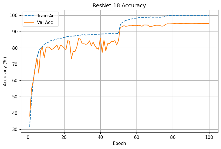
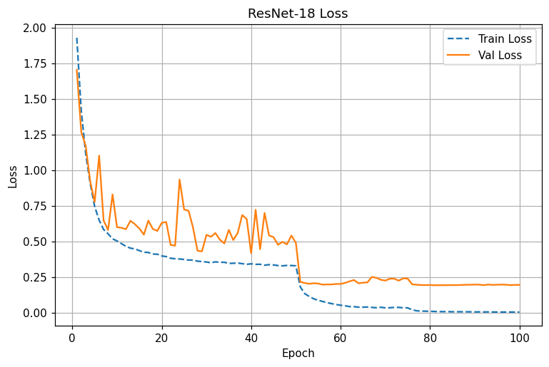
ResNet-18 : LR 스텝(50,75)에 맞춰 loss 급락 및 acc 급상승. 80에폭 이후 94.7~95.0%에 안정 수렴


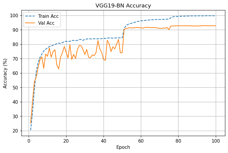
VGG19-BN: 동일 스케줄에서도 변동성 높음, 후반 개선 둔화. 최종 92.7~92.9% 근처 수렴


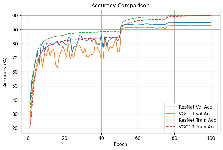
동일 조건 비교: ResNet은 전 구간에서 낮은 Val loss와 높은 Val acc를 유지. LR 스텝 직후 개선 폭이 VGG보다 큼

정성 해석
- 초기(1~10에폭): 둘 다 급격한 손실 감소. ResNet이 조금 더 빠르게 val acc 80% 안착.
- 중기(10~50에폭): VGG는 val 변동성이 큼(오버피팅 시그널), ResNet은 변동폭 작음.
- LR step @50: 두 모델 모두 성능 점프. ResNet은 0.20대 val loss, 93%+로 치고 올라감.
- 후기(80~100에폭): ResNet은 95% 근처에서 plateau, VGG는 92~93%에서 정체.
3.3 왜 ResNet이 더 잘 학습되는가 (실증 + 원리)
- Identity Shortcut으로 안정적 역전파
- 합연산을 통한 직접 경로가 항상 열려 있어 깊이가 늘어나도 gradient 소실/폭주가 크게 억제됨.
- 네 곡선에서 확인되는 Val loss 하한과 수렴 속도 차이가 이를 반영.
- 잔차 학습(Residual) = 탐색 공간 축소
- H(x)를 직접 학습하는 대신 F(x)=H(x)-x만 학습 → identity 주변의 작은 보정을 찾는 문제로 단순화.
- 스케줄 스텝 이후 ResNet의 빠른 재수렴이 이를 실증.
- 용량/일반화 균형
- ResNet-18 11.17M vs VGG19-BN 38.96M → 동일 증강/정규화에서 ResNet의 일반화 오차가 낮아지는 경향.
- 표에서 loss 격차(0.19 vs 0.33)와 정확도 격차(+2.12pp)로 드러남.
- 표현력 낭비 최소화
- Block 단위로 “필요한 변화만 추가”하므로 과도한 특성 중복/공유가 줄어들고 효율적 표현을 학습.
4. 결론
- 동일한 조건에서 직접 구현한 ResNet-18은 VGG19-BN 대비 테스트 정확도 +2.12pp (94.99% vs 92.87%), 손실 낮음(0.1937 vs 0.3345), 파라미터 3.5× 적음.
- 곡선 분석에서 확인되듯, Residual 연결이 최적화와 일반화 모두에 실질적 이득을 제공한다.
'논문 리뷰' 카테고리의 다른 글
| [논문 리뷰] Deep Residual Learning for Image Recognition 논문 과제 (1) | 2025.08.07 |
|---|---|
| AlexNet 논문에서 ReLU를 사용한 이유 직접 실험해보기, Sigmoid 함수의 정확도는 왜 이렇게 나왔을까? (3) | 2025.08.04 |
| AlexNet 아키텍처 직접 구현 및 CPU vs GPU 실험 (정확도가 다르게 나온 이유?) (2) | 2025.08.04 |
| ImageNet Classification with Deep Convolutional Neural Networks(2012) | AlexNet 논문 핵심 내용 요약 (4) | 2025.08.03 |
| 딥러닝 논문 가이드 _ 딥러닝 전체 (1) | 2025.08.03 |