붓꽃 데이터셋을 사용한 Classification 실습 분석
1. 코드의 목적과 역할 분석
Scikit-learn의 붓꽃(Iris) 데이터셋을 사용해 분류를 위한 데이터 전처리 + 시각화를 하고,
데이터를 머신러닝 모델에 맞체 훈련(train) 데이터와 테스트(test) 데이터로 분리하는 것
* 붓꽃 데이터 셋 : 꽃받침(sepal), 꽃잎(petal)의 길이와 너비 정보를 바탕으로 붓꽃 품종을 구분하는 대표적인 분류 문제용 데이터 셋
2. 필수 라이브러리
pandas : 데이터 전처리 및 분석용
numpy : 수치 연산 및 행렬 연산
scikit-learn : 머신러닝 데이터셋 및 데이터 분할 (train_test_split)
matplotlib/seaborn : 데이터 시각화
3. 주요 기능
1. Iris 데이터셋 로드 및 데이터 프레임 변환
2. 데이터 전처리 (컬럼명 변경, 중복 데이터 제거)
3. 데이터 분포 시각화 (displot, pariplot)
4. 훈련데이터, 테스트 데이터 분할
4. 코드 뜯어먹기
1. 필수 라이브러리 import
import pandas as pd        # 데이터 분석용 (데이터프레임 생성, 전처리)
import numpy as np         # 수치 계산 및 배열 처리를 위한 라이브러리
from sklearn import datasets  # 머신러닝용 데이터셋을 불러오기 위한 라이브러리
2. Iris 데이터셋 로드
iris = datasets.load_iris() # 사이킷런 내장 데이터셋인 Iris 데이터셋 로딩
print(iris)
print(type(iris))

========= 출력 예시 =========
{'data': array([[5.1, 3.5, 1.4, 0.2],
       [4.9, 3. , 1.4, 0.2],
       [4.7, 3.2, 1.3, 0.2],
       [4.6, 3.1, 1.5, 0.2],
       [5. , 3.6, 1.4, 0.2],
       [5.4, 3.9, 1.7, 0.4],
       [4.6, 3.4, 1.4, 0.3],
       [5. , 3.4, 1.5, 0.2],
....
 [6.7, 3. , 5.2, 2.3],
       [6.3, 2.5, 5. , 1.9],
       [6.5, 3. , 5.2, 2. ],
       [6.2, 3.4, 5.4, 2.3],
       [5.9, 3. , 5.1, 1.8]]), 'target': array([0, 0, 0, 0, 0, 0, 0, 0, 0, 0, 0, 0, 0, 0, 0, 0, 0, 0, 0, 0, 0, 0,
       0, 0, 0, 0, 0, 0, 0, 0, 0, 0, 0, 0, 0, 0, 0, 0, 0, 0, 0, 0, 0, 0,
       0, 0, 0, 0, 0, 0, 1, 1, 1, 1, 1, 1, 1, 1, 1, 1, 1, 1, 1, 1, 1, 1,
       1, 1, 1, 1, 1, 1, 1, 1, 1, 1, 1, 1, 1, 1, 1, 1, 1, 1, 1, 1, 1, 1,
       1, 1, 1, 1, 1, 1, 1, 1, 1, 1, 1, 1, 2, 2, 2, 2, 2, 2, 2, 2, 2, 2,
       2, 2, 2, 2, 2, 2, 2, 2, 2, 2, 2, 2, 2, 2, 2, 2, 2, 2, 2, 2, 2, 2,
       2, 2, 2, 2, 2, 2, 2, 2, 2, 2, 2, 2, 2, 2, 2, 2, 2, 2]), 'frame': None, 'target_names': array(['setosa', 'versicolor', 'virginica'], dtype='<U10'), 'DESCR': '.. _iris_dataset:\n\nIris plants dataset\n--------------------\n\n**Data Set Characteristics:**\n\n:Number of Instances: 150 (50 in each of three classes)\n:Number of Attributes: 4 numeric, predictive attributes and the class\n:Attribute Information:\n    - sepal length in cm\n    - sepal width in cm\n    - petal length in cm\n    - petal width in cm\n    - class:\n            - Iris-Setosa\n            - Iris-Versicolour\n            - Iris-Virginica\n\n:Summary Statistics:\n\n============== ==== ==== ======= ===== ====================\n                Min  Max   Mean    SD   Class Correlation\n============== ==== ==== ======= ===== ====================\nsepal length:   4.3  7.9   5.84   0.83    0.7826\nsepal width:    2.0  4.4   3.05   0.43   -0.4194\npetal length:   1.0  6.9   3.76   1.76    0.9490  (high!)\npetal width:    0.1  2.5   1.20   0.76    0.9565  (high!)\n============== ==== ==== ======= ===== ====================\n\n:Missing Attribute Values: None\n:Class Distribution: 33.3% for each of 3 classes.\n:Creator: R.A. Fisher\n:Donor: Michael Marshall (MARSHALL%PLU@io.arc.nasa.gov)\n:Date: July, 1988\n\nThe famous Iris database, first used by Sir R.A. Fisher. The dataset is taken\nfrom Fisher\'s paper. Note that it\'s the same as in R, but not as in the UCI\nMachine Learning Repository, which has two wrong data points.\n\nThis is perhaps the best known database to be found in the\npattern recognition literature.  Fisher\'s paper is a classic in the field and\nis referenced frequently to this day.  (See Duda & Hart, for example.)  The\ndata set contains 3 classes of 50 instances each, where each class refers to a\ntype of iris plant.  One class is linearly separable from the other 2; the\nlatter are NOT linearly separable from each other.\n\n.. dropdown:: References\n\n  - Fisher, R.A. "The use of multiple measurements in taxonomic problems"\n    Annual Eugenics, 7, Part II, 179-188 (1936); also in "Contributions to\n    Mathematical Statistics" (John Wiley, NY, 1950).\n  - Duda, R.O., & Hart, P.E. (1973) Pattern Classification and Scene Analysis.\n    (Q327.D83) John Wiley & Sons.  ISBN 0-471-22361-1.  See page 218.\n  - Dasarathy, B.V. (1980) "Nosing Around the Neighborhood: A New System\n    Structure and Classification Rule for Recognition in Partially Exposed\n    Environments".  IEEE Transactions on Pattern Analysis and Machine\n    Intelligence, Vol. PAMI-2, No. 1, 67-71.\n  - Gates, G.W. (1972) "The Reduced Nearest Neighbor Rule".  IEEE Transactions\n    on Information Theory, May 1972, 431-433.\n  - See also: 1988 MLC Proceedings, 54-64.  Cheeseman et al"s AUTOCLASS II\n    conceptual clustering system finds 3 classes in the data.\n  - Many, many more ...\n', 'feature_names': ['sepal length (cm)', 'sepal width (cm)', 'petal length (cm)', 'petal width (cm)'], 'filename': 'iris.csv', 'data_module': 'sklearn.datasets.data'}
<class 'sklearn.utils._bunch.Bunch'>

(120, 4)
(30, 4)
(120,)
(30,)
3. 데이터 프레임 변환 후 확인
# 데이터프레임 변환 후 확인
df_iris = pd.DataFrame(data=iris.data, columns=iris.feature_names) #bunch 타입이기 때문에 지정해줘야함.
df_iris.info()

# key 확인
print(iris.keys())

====== 출력 예시 ======
<class 'pandas.core.frame.DataFrame'>
RangeIndex: 150 entries, 0 to 149
Data columns (total 4 columns):
 #   Column             Non-Null Count  Dtype
---  ------             --------------  -----
 0   sepal length (cm)  150 non-null    float64
 1   sepal width (cm)   150 non-null    float64
 2   petal length (cm)  150 non-null    float64
 3   petal width (cm)   150 non-null    float64
dtypes: float64(4)
memory usage: 4.8 KB

dict_keys(['data', 'target', 'frame', 'target_names', 'DESCR', 'feature_names', 'filename', 'data_module'])
(120, 4)
(30, 4)
(120,)
(30,)

=> 데이터 셋을 훈련용/테스트용으로 나눈 후의 출력
- Iris['data'] : 데이터셋에서 특성 데이터를 의미 -> 컬럼명을 ['feature_names']로 지정해줌
- 데이터프레임 형태가 아닌 딕셔너리 형태라면 info()가 찍히지 않음
=> 150건의 데이터가 있고, 4개의 컬럼이 있음.
+) keys()를 찍어보는 이유?
iris 처럼 생긴 딕셔너리 또는 Bunch 객체를 다룰 때 그 안에 어떤 정보가 들어있는지 구조를 모를 경우
-> 이 객체에서 어떤 데이터를 꺼내 쓸 수 있지? 를 빠르게 파악하려고 찍는 것 (분석에 필요한 x와 y를 골라내는 데 쓰임)
dict_keys([
  'data',         # X값 (독립 변수, 특성 데이터)-꽃잎 길이, 꽃받침 너비 등 수치
  'target',       # y값 (종속 변수, 레이블)- 붓꽃 종류 (0,1,2)
  'frame',        # pandas DataFrame (있을 수도, 없을 수도 있음)
  'target_names', # 레이블 이름 (예: ['setosa', 'versicolor', 'virginica'])
  'DESCR',        # 설명문 (데이터셋 전체 설명)
  'feature_names',# 각 특성 이름
  'filename'      # 데이터셋 파일 경로
])
4. 데이터셋 정보, 특성(변수)명 출력, 특성(feature) 데이터
# 데이터셋 정보
print(iris['DESCR'])

# 특성(변수)명 출력
print(iris.feature_names)
print(iris['feature_names'])

# 특성(feature) 데이터 (대문자 X)
# = 독립 변수 (분류를 확정하기 위한 데이터)
print(iris['data'])
features = iris['data']
print(features[:5])

# 레이블(Label) 데이터 (소문자 y)
# = 종속 변수 (분류)
print(iris['target'])

===== 출력 결과 =====
.. _iris_dataset:

Iris plants dataset
--------------------

**Data Set Characteristics:**

:Number of Instances: 150 (50 in each of three classes)
:Number of Attributes: 4 numeric, predictive attributes and the class
:Attribute Information:
    - sepal length in cm
    - sepal width in cm
    - petal length in cm
    - petal width in cm
    - class:
            - Iris-Setosa
            - Iris-Versicolour
            - Iris-Virginica

:Summary Statistics:

============== ==== ==== ======= ===== ====================
                Min  Max   Mean    SD   Class Correlation
============== ==== ==== ======= ===== ====================
sepal length:   4.3  7.9   5.84   0.83    0.7826
sepal width:    2.0  4.4   3.05   0.43   -0.4194
petal length:   1.0  6.9   3.76   1.76    0.9490  (high!)
petal width:    0.1  2.5   1.20   0.76    0.9565  (high!)
============== ==== ==== ======= ===== ====================

:Missing Attribute Values: None
:Class Distribution: 33.3% for each of 3 classes.
:Creator: R.A. Fisher
:Donor: Michael Marshall (MARSHALL%PLU@io.arc.nasa.gov)
:Date: July, 1988

The famous Iris database, first used by Sir R.A. Fisher. The dataset is taken
from Fisher's paper. Note that it's the same as in R, but not as in the UCI
Machine Learning Repository, which has two wrong data points.

This is perhaps the best known database to be found in the
pattern recognition literature.  Fisher's paper is a classic in the field and
is referenced frequently to this day.  (See Duda & Hart, for example.)  The
data set contains 3 classes of 50 instances each, where each class refers to a
type of iris plant.  One class is linearly separable from the other 2; the
latter are NOT linearly separable from each other.

.. dropdown:: References

  - Fisher, R.A. "The use of multiple measurements in taxonomic problems"
    Annual Eugenics, 7, Part II, 179-188 (1936); also in "Contributions to
    Mathematical Statistics" (John Wiley, NY, 1950).
  - Duda, R.O., & Hart, P.E. (1973) Pattern Classification and Scene Analysis.
    (Q327.D83) John Wiley & Sons.  ISBN 0-471-22361-1.  See page 218.
  - Dasarathy, B.V. (1980) "Nosing Around the Neighborhood: A New System
    Structure and Classification Rule for Recognition in Partially Exposed
    Environments".  IEEE Transactions on Pattern Analysis and Machine
    Intelligence, Vol. PAMI-2, No. 1, 67-71.
  - Gates, G.W. (1972) "The Reduced Nearest Neighbor Rule".  IEEE Transactions
    on Information Theory, May 1972, 431-433.
  - See also: 1988 MLC Proceedings, 54-64.  Cheeseman et al"s AUTOCLASS II
    conceptual clustering system finds 3 classes in the data.
  - Many, many more ...
=> iris 데이터에 대한 상세 설명 확인 가능
핵심 내용 :
- 전체 150개 샘플, 클래스당 50개, 특성은 4개(예측에 쓰이는 수치형)
- 각 특성이 무엇을 의미하는지, 클래스(label)은 3가지 붓꽃 종류임
- 요약 통계 (평균, 표준편차, 특성과 레이블의 상관관계) -> 특히 petal계열은 상관계수가 높기 때문에 분류 성능에 매우 중요한 특성
- 결측치 여부 : 없음 (바로 모델링 가능)
['sepal length (cm)', 'sepal width (cm)', 'petal length (cm)', 'petal width (cm)']
['sepal length (cm)', 'sepal width (cm)', 'petal length (cm)', 'petal width (cm)']

[[5.1 3.5 1.4 0.2]
 [4.9 3.  1.4 0.2]
 [4.7 3.2 1.3 0.2]
 [4.6 3.1 1.5 0.2]
 [5.  3.6 1.4 0.2]
 ...
  [4.6 3.1 1.5 0.2]
 [5.  3.6 1.4 0.2]]


[0 0 0 0 0 0 0 0 0 0 0 0 0 0 0 0 0 0 0 0 0 0 0 0 0 0 0 0 0 0 0 0 0 0 0 0 0
 0 0 0 0 0 0 0 0 0 0 0 0 0 1 1 1 1 1 1 1 1 1 1 1 1 1 1 1 1 1 1 1 1 1 1 1 1
 1 1 1 1 1 1 1 1 1 1 1 1 1 1 1 1 1 1 1 1 1 1 1 1 1 1 2 2 2 2 2 2 2 2 2 2 2
 2 2 2 2 2 2 2 2 2 2 2 2 2 2 2 2 2 2 2 2 2 2 2 2 2 2 2 2 2 2 2 2 2 2 2 2 2
 2 2]

 (120, 4)
(30, 4)
(120,)
(30,)
5. 컬럼명에서 단위(cm) 제거
df.columns = ['sepal_length', 'sepal_width', 'petal_length', 'petal_width']
print(df.head())

===== 출력 =====

  sepal_length  sepal_width  petal_length  petal_width
0           5.1          3.5           1.4          0.2
1           4.9          3.0           1.4          0.2
2           4.7          3.2           1.3          0.2
3           4.6          3.1           1.5          0.2
4           5.0          3.6           1.4          0.2
6. target 변수 추가 (종속)
df['target'] = iris['target']
print(df.tail())


==== 출력 ====
     sepal_length  sepal_width  petal_length  petal_width  target
145           6.7          3.0           5.2          2.3       2
146           6.3          2.5           5.0          1.9       2
147           6.5          3.0           5.2          2.0       2
148           6.2          3.4           5.4          2.3       2
149           5.9          3.0           5.1          1.8       2
7. 중복 데이터 확인
print(df.duplicated().sum())  #합계 출력
print(df.loc[df.duplicated(keep=False)]) #중복된 데이터 행을 전부 출력하여 확인

==== 출력 ====
1

sepal_length  sepal_width  petal_length  petal_width  target
101           5.8          2.7           5.1          1.9       2
142           5.8          2.7           5.1          1.9       2
8. 중복 데이터 제거 후 확인
df = df.drop_duplicates()
print(df.duplicated().sum()) # 중복데이터의 합
9. 시각화 라이브러리 임포트 및 설정
import matplotlib.pyplot as plt #시각화를 위한 기본적인 라이브러리 임포트
import seaborn as sns #고급 시각화를 지원하는 seaborn 라이브러리 임포트

#한글 폰트 설정
plt.rc('font', family='Malgun Gothic')

#캔버스 사이즈 설정
plt.rcParams['figure.figsize'] = (12, 10)
10. 데이터 분포 시각화 (displot, pairplot)
displot 그리기 : 데이터 분포 확인에 사용되는 그래프
x : x축에 표시할 특성, kind : 그래프 종류, hue : 범례, data : 데이터 프레임
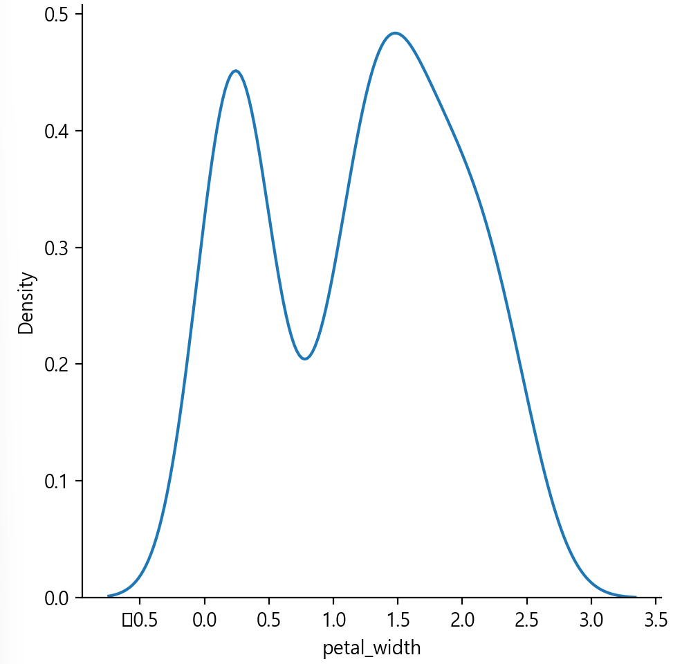
# petal_width 전체 분포
클래스 구분 없이 petal_width의 전체 분포를 보여줌

sns.displot(x='petal_width', kind='kde', data=df)
plt.show()

=>
분포가 두 개의 봉우리 (bimodal) 형태 -> 데이터가 2~3개의 뚜렷한 집단으로 나뉨을 암시
실제로 setosa는 petal_width가 거의 0.2~0.6 사이에 몰려있고 나머지는 더 넓은 값대를 가짐
petal_width가 클수록 Virginica일 확률이 높고, 작으면 Setosa일 확률이 높음
결론 : 분리 성능이 매우 우수한 변수
실제로 상관계수도 0.9565로 target과 거의 직결


===================

#sepal_width(꽃받침 너비)의 밀도 곡선을 품종(target)별로 시각화
sns.displot(x='sepal_width', kind='kde', hue='target', data=df)
plt.show()
=>
0(setosa)의 분포는 오른쪽으로 치우쳐 있음 -> 평균적으로 꽃받침이 더 넓다
1, 2 (Versicolour, Virginica)는 분포가 거의 겹쳐 있음 -> 잘 구분 안됨
결론 : sepal_width는 setosa는 잘 구분하지만, 나머지 둘은 구분 어려움
이 특성은 완전한 분리에는 부적절함 (분류 성능 제한) target과의 상관관계도 낮은 편

=> petal_width, petal_length는 분류 모델에 중요한 입력 변수로 사용해야 함
pairplot 그리기 : 데이터 프레임의 각 변수들 간의 쌍(pair)들의 관계 확인에 사용
순서 : 데이터프레임, 범례, 그래프 높이, 그래프 종류
sns.pairplot(df, hue='target', height=3.5, diag_kind='kde')
plt.show()
+) pariplot : 변수들 간의 관계를 한 눈에 보기 위해 구성된 격자형 시각화
1. 대각선 (diagonal) - KDE 곡선 (밀도 선 그래프) : 클래스 간 분포 차이를 파악 (분리 가능성 확인)
diag_kind='kde' 옵션을 줬기 때문에 대각선에는 각 변수의 분포 곡선(선 그래프 형태) 이 그려짐
히스토그램 대신 커널 밀도 추정(KDE) 그래프
예: sepal_length, sepal_width, petal_length, petal_width 각각의 단변량 분포
왜 선 그래프인가?
diag_kind='kde' 옵션을 주었기 때문. 기본은 hist (막대)이고, kde는 부드러운 곡선으로 밀도 분포를 그림
(1) sepat_length (첫 번째 대각선 셀)
0번은 짧은 길이에 몰려있음, 2번은 긴 길이에 몰려있음, 1번은 중간 길이
=> 세 클래스가 약간 겹치지만 비교적 나눠져 있음
(2) sepal_width(두 번째 대각선 셀)
0번만 오른쪽으로 치우침 -> 꽃받침 너비가 큼, 나머지 클래스는 왼쪽에 몰림
=> 0번은 구분 가능하지만 나머지는 겹침
(3) petal_length(세 번째 대각선 셀)
0번은 매우 짧은 꽃잎, 나머지는 길지만 구간이 다름
=> 셋다 명확히 분리됨 (거의 안겹침 ) => 머신러닝 모델에 매우 유리한 특성
(4) petal_width(네 번째 대각선 셀)
가장 극단적으로 분포 차이가 크다.
=> 분류에서 결정적 역할, 상관계수도 0.95 이상으로 가장 높음
2. 비대각선 - 산점도 (Scatter Plot) : 변수 쌍 중 어떤 조합이 클래스를 잘 나누는지 시각적으로 판단
x,y축이 서로 다른 두 변수일 때는 산점도를 그린다.
점들은 각 데이터 샘플을 의미하고, hue=target 옵션으로 색깔이 클래스(종)에 따라 달라짐
왜 산점도인가?
두 변수간의 관계성(상관관계, 분리 가능성)을 시각적으로 보기 위해 사용됨
=> 특히 petal_length vs petal_width 조합은 거의 완벽하게 3종을 나눔
11. Train/Test 데이터 셋 분할
from sklearn.model_selection import train_test_split #데이터셋을 나누기 위한 함수 임포트

# 특성(feature) 데이터와 레이블(label)을 각각 변수에 담기
iris_data = iris.data
iris_label = iris.target
X_train, X_test, y_train, y_test \
    = train_test_split(
    iris_data, # 훈련데이터
          iris_label, # 특성명
          test_size = 0.2, # 분리비율 : 80%는 훈련용, 20%는 테스트용
          random_state = 7 # 데이터 분리할때 어떤 데이터들을 추출해서 분리할지를
                           # 랜덤하게 결정하기 위한 랜덤 시드값
                           # 랜덤 시드값이 같으면 항상 같은 분리를 함
+)random_state의 역할 : 재현 가능한 (항상 똑같은) 데이터 분리 결과를 얻기 위해 사용되는 설정값
: train과 test 데이터를 나눌 때 사용하는 랜덤 추출 방식의 '시드(seed)'를 고정
- random_state 값을 고정하면, 항상 같은 방식으로 데이터를 나눔
- 반대로 값을 안 주면, 실행할 때마다 train/test가 다르게 섞여 나뉨
중요한 이유 :
1. 실험 재현성 확보 : 항상 같은 데이터 분할을 사용해야 모델 성능 비교가 정확함
2. 팀프로젝트나 논문 제출 시 필수 : 누가 실행하더라도 결과가 같도록 보장해야함.
언제 어떤 값을 쓰나?
값은 아무 숫자나 가능
중요한 것 고정된 값만 쓰면 항상 같은 결과가 나온다는 것
random_state=42는 많이 쓰는 관례적인 숫자
Q. 고정된 값을 사용하면 사실상 조작 아닐까...?
k-fold cross-validation 사용해서 여러번 나눠 평균 성능을 보는 방식. 시드 고정 x
다양한 random_state 값으로 테스트 후 평균 성능 발표 ( 예: random_state = 0~9로 10번 실험 후 평균값 계산)
12. 분할된 데이터 확인하기
print(X_train.shape) # 데이터의 모양=차원, 2차원(120, 4):120행 4열
print(X_test.shape) # 2차원(30, 4): 30행 4열
print(y_train.shape) # 1차원(120, ) : 120개
print(y_test.shape) # 1차원(30, ) : 30개
5. 분석적 인사이트
4개의 특성 (꽃받침 길이/너비, 꽃잎 길이/너비)을 기반으로 3가지 붓꽃 품종을 분류할 수 있다.
pairplot과 displot을 통해 특성 간 데이터 분포와 상관관계를 직관적으로 파악하여 효과적인 특성과 전처리 가능
데이터 분할 시 random_state를 사용하여 모델 학습을 반복할 때마다 일관된 결과를 얻을 수 있음.
'Data Analysis' 카테고리의 다른 글
| Classification (분류 알고리즘) 개념 (5) | 2025.06.08 |
|---|---|
| Linear Regression (선형 회귀) (1) | 2025.06.08 |
| 머신러닝(Machine Learning), Big Data, AI의 기초 개념 (4) | 2025.06.08 |
| 상관분석, 상관행렬(correlation matrix), heatmap (3) | 2025.06.04 |
| 가설검정, t-검정, 상관분석, 유의확률, scipy (2) | 2025.06.02 |